Finding eclipsing binaries in NSVS data

by Patrick Wils (email:

)

Variability searches and the NSVS

The Northern Sky Variability Survey (NSVS in short) was a CCD survey of the Northern sky using the first generation Robotic Optical Transient Search Experiment (ROTSE-I). See their public data release paper for complete details. All the NSVS data can be queried online. Variability searches for red long period variables (Williams et al., 2004), Cepheids (Wils & Greaves, 2004), RR Lyrae stars (Wils et al., 2006 and Kinemuchi et al., 2006) and contact binaries (Gettel et al., 2006). Also the COROT fields were searched for all types of variable stars (Benk & Csubry, 2007). Although eclipsing binaries were found as "by-products" of other searches (Otero et al., 2004), no systematic search for detached or semi-detached eclipsing binaries has been performed in the entire NSVS database. As eclipsing binaries consititute a large fraction of all variable stars, very likely a large number have not yet been discovered, especially in the region of the sky North of declination +28 degrees, which has not been covered by ASAS so far.

Statistical methods used when searching for eclipsing binaries

There are several ways to start looking for variable stars. Usually stars are selected with more "scatter" in their data (a larger standard deviation) than what is normal for their magnitude. This can be done constructing SQL statements and using the NSVS online interface. It is a rather tedious work and most of all, in order not to miss real variables, the cutoff values must be chosen rather generously, resulting in a lot of false alarms, and numerous non-variable stars to be checked. Especially a low amplitude detached eclipsing binary may only have a few fainter than normal data points during eclipses, with little influence on the standard deviations. It may therefore go undetected using this technique, because of erroneous outlier points. In a plot of standard deviation against median magnitude for one of the NSVS fields (Fig. 1), it can be seen that most known variables (green triangles) have very large standard deviation.

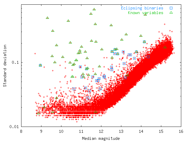
Fig. 1: Standard deviation (logarithmic sacle) plotted against median magnitude for all stars with more than 50 data points from NSVS field 016b.

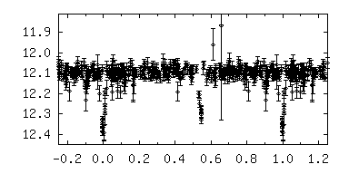
However, in general eclipsing binaries (blue squares) lie much closer to the band of stars with normal scatter. One may also remove the faintest and brightest data points from the data set to deal with those possibly erroneous outlier points, however in the case of eclipsing binaries this may remove most of the real eclipse points as well (see the data of XZ Cam for a typical light curve of a detached eclipsing binary in the NSVS database). Furthermore, working with the standard deviation alone does not discriminate between variable star types, and one may recover a lot of previously discovered variables of other types. So other statistics are required to differentiate.

A lot of the principles mentioned in the following sections are applicable not only to the NSVS database, but to other surveys as well. Note that the condition for the standard deviation to be higher than average will not be used here. Only specific properties of the magnitude distribution will be used to find eclipsing binaries.

Statistic EA₁

A typical EA type eclipser has a very specific magnitude distribution in survey data. Since generally up to five observations were made per night, several nights in a row or with several nights between them, most of the observations will be from a star at maximum, with only a few observations near minimum or on the ascending or descending branch. This means that the median of the magnitudes (the "middle" magnitude) will be near maximum. Also the difference between the median and the brightest point will be much smaller than between the faintest point and the median. This is one condition that can be used to distinguish eclipsing binaries from constant stars and other variable types. Instead of taking the brightest and faintest point the 2nd and 98th percentile P₂ and P₉₈ are used to remove possible erroneous outliers that might make the calculated value unusable. The first condition is then:

EA₁ = (P₉₈ - median)/(median - P₂) >= 2

The value of 2 was chosen so that it includes the large majority of eclipsing binaries and excludes a large fraction of other variable star types. A plot for this statistic against median magnitude is given in Fig. 2.

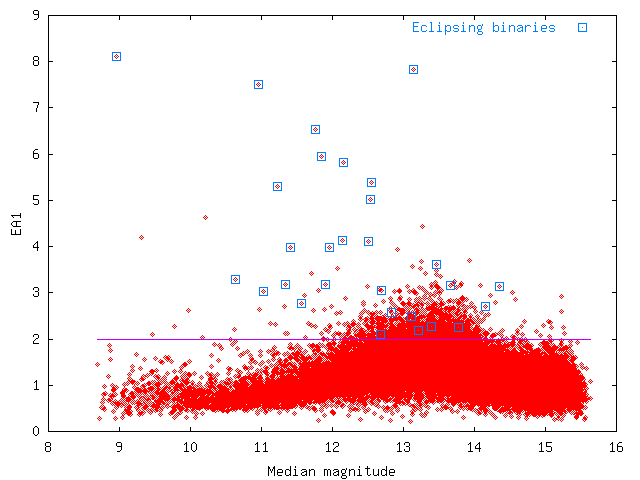Fig. 2: EA₁ plotted against median magnitude for all stars with more than 50 data points from NSVS field 016b. Eclipsing binaries and the cutoff value used in this study are indicated as well.

The remaining cutoffs where derived from looking for eclipsing binaries in twelve NSVS fields placed in different locations around the sky. Optimal values were chosen to remove most of the false alarms, while keeping all or almost all the real variables. Relaxing the conditions may still reveal new eclipsing binaries but at the cost of many more stars to be checked in vain.

Skewness

Another measure of "spending more time near maximum than near minimum" is skewness γ₁. A magnitude distribution with zero skewness is symmetric around the mean. Those with positive skewness have more values near the bright end. The calculation of skewness involves all the data, not just magnitude ranges as in EA₁. Most of the stars excluded by a condition on EA₁ will also be excluded by a skewness condition and vice versa, but some weird magnitude distributions, usually resulting from "problematic" stars like unresolved doubles, will be dropped from the possible candidates by considering both conditions. The following cutoff was chosen:

γ₁ >= 0.8

This excludes some EW type eclipsing binaries, but since systematic searches have already been done for those, the number of stars of this type left undiscovered may be small.

Mean of squared successive differences

The mean of squared differences between successive magnitudes (with the magnitudes ordered according to the time of observation, as is the case in the NSVS data files) is a measure of monotonous variation of the star. With the MSSD statistic calculated in the form given by Wils et al. (2006), a value near 1 means the star brightened or faded gradually during the observations and will almost certainly be a long period variable. Values much smaller than 1 (including negative values) indicate more erratic variation, which is exactly the expected behavior for eclipsing binaries in view of the survey's observational cadence. A good cutoff value is:

MSSD <= 0.75

Note that this might exclude a number of eclipsing binaries with a period very close to (an integer fraction of) one (sidereal) day. Taking observations exactly one day apart might mimick the behaviour of a long period (eclipsing) variable, see UW Boo with a period of 1.0047108 days for an example (note that UW Boo does satisfy the above condition).

Stars not satisfying the MSSD condition, and certainly those with MSSD >= 0.9, will very likely be long period variables, as is the case for XY Cam.

Statistics EA₂ and EA₃

The above conditions applied to NSVS data will still turn up a lot of constant stars, mostly because of questionable data (often near the NSVS magnitude limit). When studying these cases it was found that the uncertainties and standard deviations for parts of the magnitude distributions were unusually large. For instance, one expects the standard deviation of the magnitudes fainter than the median to be larger than the standard deviation for the brighter data points: fainter points always show larger uncertainty, but most importantly an eclipsing binary shows most of its variation near minimum (while in eclipse) and almost no variation near maximum:

EA₂ = standard deviation faint points/standard deviation bright points >= 2

Fig. 3 shows how this statistic is related to median magnitude.

Fig. 3: Same as Fig. 2, but this time for EA₂.

Combining EA₁ and EA₂ reveals that a large fraction of the false eclipsers are excluded by applying these cutoffs (see Fig. 4).

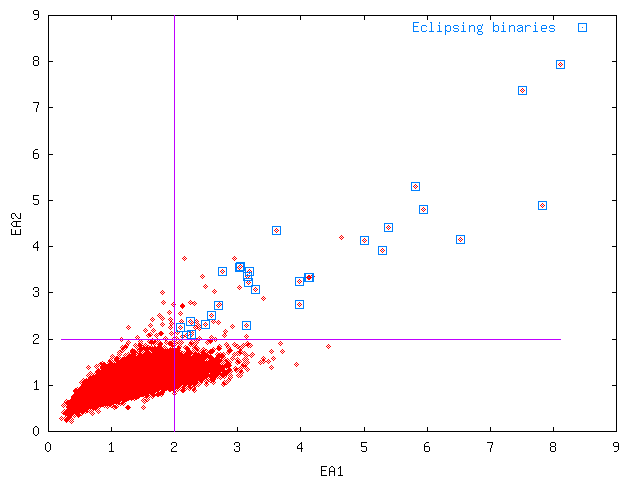Fig. 4: EA₂ plotted against EA₁ for NSVS field 016b. The constraints remove most of the false alarms, while keeping all real eclipsing variables in this field.

Finally the uncertainties of the NSVS data are expected to be larger in the faint range than in the bright range. When this fails there are likely some problems with the data. For an exact definition of EA₃ see the Perl script provided with this article. The cutoff value was chosen to be:

EA₃ >= 0.8

A practical method

Instead of using the NSVS SQL interface to do these calculations, it is much more efficient to download the zipped data for an entire field from the NSVS ftp site and calculate the statistics for each star based on those files. The files in question are called "skydotID_NNNX.sql.gz" with NNN between 001 and 161 and X = a, b, c or d, representing the 644 fields of the sky that NSVS observed. Each field measures approximately eight by eight degrees, with some overlap between fields. The list of fields is given here. Depending on the number of frames and the number of objects, these files are up to 170 Mb large, at low declinations they are generally much smaller, some less than 1 Mb. The total size is about 30 Gb. Fortunately there is no need to unzip the files. The Perl script listed here will take one such file and calculate the statistics mentioned above. It is called like this from a command line:

perl nsvsstats.pl NNNX >NNNX.txt

with NNNX the NSVS field name. The zipped NSVS data file should be in the current directory.

Knowledge of Perl is not required to use this script, only a Perl runtime is needed, e.g. ActivePerl provided by ActiveState for a number of operating systems. The output of the script is a tab delimited list of NSVS identification numbers and the following statistics on magnitude: maximum, average, minimum, number, 2nd percentile, median, 98th percentile, standard deviation, skewness, kurtosis, mean of successive squared differences, and the three EA_i indexes defined above. The data are filtered on the flags (mask = 15636) described in Wils et al. (2006), and only objects with 50 or more data points are listed. Standard spreadsheet programs can then be used to filter the objects. Note that these statistics are not only useful for finding eclipsing binaries, but may be used for other purposes as well.

Period determination

Despite all the imposed conditions, not all of the selected objects will be real variables. Depending on the field (Galactic fields will probably suffer most), 40 to 95% of the objects satisfying the above conditions will be "false alarms", constant stars with erroneous faint data points due to cosmic rays, a close companion, bad weather, etc. Especially the "c" camera produces much more false candidates. To make sure the the stars selected above are really eclipsing binaries, their period needs to be found. The NSVS data files do not contain the time of observation, only the frame id. So if one wants to determine the period this frame id has to be replaced by the corresponding time, preferably the Heliocentric Julian Date (HJD). The easiest way to do is to download the NSVS frames table (a 10 Mb file) and convert the frame id's using the Perl script nsvsframes.pl. This will create a binary file called "Skydot-Frames.bin" with HJD values that should be kept in the same directory as the NSVS data files. Note that nsvsframes.pl uses the Perl module Astro::Time::HJD to calculate heliocentric times. This module has likely not been installed by default with the Perl distribution. You can also download the file Skydot-Frames.bin here.

The script nsvsstats.pl will use the binary file "Skydot-Frames.bin" to create tab delimited data files for each of the objects satisfying the conditions determined in the previous section. These data files are called NSVSxxx.dat with "xxx" the NSVS id of the object. They contain lines with HJD - 2450000, the magnitude, the uncertainty on the magnitude and the flag values for the object in question. Those files may then be used by period determination software.

For EA type eclipsing binaries however the usual period search methods may regularly fail. It is often the case that most observations are made near maximum with little scatter. Only a few faint points are available, with large periods in between. Most of the information is therefore in the times of minimum, not necessarily in the magnitudes. Using a trial period, an integer number of cycles between the times of minimum can be determined and a least squares fit done to improve that period. This can be repeated for a number of trial periods, the best periods selected and verified in a phase plot with all the data.

To facilitate searches based on the above method, the Excel workbook OCEASE.xls was developed. Here is how it works (see Fig. 5): Fill in the list of minima in the A column of the "Calculate" sheet. Make sure there are at least three times of minimum and that no two lines refer to the same minimum. Put the smallest period you want to test in cell E2 and the largest one in E7 (or leave the latter blank for testing the largest possible period). Cell E6 contains the number of minima per cycle (either 1 or 2). Generally keep it equal to 1, so that for e.g. in the case of EW variables half the real period will be found (remember to set the period limits accordingly). Don't change other cells, and press the "Calculate" button. It will test all possible cycle counts (least squares fitting) over the entire timespan. When it has finished, the best period found is shown in E4, the epoch in E3.

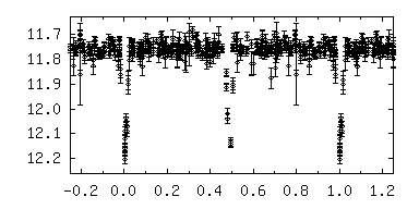
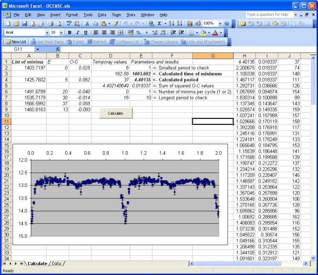Fig. 5: A screenshot of the Excel workbook, after finding the period for NSVS 6386066 = ASAS 003933+2730.5.

The other worksheet needs to contain the data for a star. The plot on the "Calculate" sheet is based on these data points. It gives a phase diagram, based on the period found. Copy the HJD values to the A column and magnitudes to column B of the "Data" sheet (this may be done with one "Select All/Copy/Paste" action from the object data files; the uncertainties will be copied to column C; don't forget to remove extra lines with data from a previous object). Make sure the phases are calculated in columns E and F for each of the points (drag the contents to the last data line if necessary).

The "Data" sheet can be used to determine the times of eclipse as well. Just sort the data in reverse order according to magnitude and select the times of the faintest points for copy in column A of the Calculate worksheet. Remove the times corresponding to the same eclipse as a previous line (e.g. data points from the same night).

With the phase plot, it is easy to see whether the period found is correct. Since the calculated period is based only on times of minimum, not on all the data, it is quite possible that the phase plot shows points at maximum near phase 0. This means that the period found is not correct, possibly too short (doubling the period might give a better result in these cases; a quick check can be done by halving the cycle count in cell D4). Therefore, after the calculation, all other periods tested are provided in the H, I and J columns with respectively the period, the sum of squared deviations (= SSD), and the cycle count over the total timespan. These are sorted in order of increasing SSD. So after the calculation, the period in E4 will be a copy of H1, the cycle count in D4 a copy of J1, and the SSD in E5 a copy of I1. If the first period is not good, try one of the others by copying one of the cycle counts from the J column into D4, or retry the calculation with other minimum and maximum limits for the period. It may also be necessary to choose a different set of times of minimum. Indeed some points may be erroneous or may be from an eccentrically placed secondary minimum. The latter may not be treated very well by the above procedure. In some cases combining the data with those from "synonyms" of the object (the same star but observed in another NSVS field and therefore with another NSVS number) may help in finding the period or improve it.

Variable star identification

The eclipsing binaries found this way will not all be new ones of course. Check the coordinates of the star by replacing "ID" in the URL "http://skydot.lanl.gov/nsvs/star.php?mask=15636&num=ID" by its NSVS number. Those coordinates can then be used in VSX to verify whether it has been found before. Note that VSX is not a complete database of all known variable stars, so the object may still have been found before. Also the object may have been found before in another field (with another number) because fields overlap to some degree and objects are numbered by field (so called NSVS synonyms).

Results so far

A list of 127 new eclipsing binaries found during this investigation in the "test" fields is given here. All stars satisfy the various cutoffs outlined above. Of those variables 106 are EA type variables, and 21 are contact systems. In addition 59 previously known eclipsing binaries were also recovered in this way (not listed), 24 EA variables and 35 contact binaries. Only 10 EA type eclipsing binaries listed in VSX with at least one data point in the NSVS database did not satisfy the cutoffs: three had less than 50 data points, another three had very noisy data, another one had no eclipses in the data and one had only one eclipse. From the remaining stars, one failed on the EA₁ restriction, and one star failed to satisfy both the EA₂ and EA₃ criteria. Therefore we can estimate that about 30% of the detached or semi-detached eclipsing binaries that have been observed by NSVS, were missed.

The table of new eclipsing binaries contains the NSVS id (with a hyperlink to the source data), the position for equinox 2000, the NSVS field, maximum and minimum magnitude (actually the 2nd and 98th percentile), an epoch of minimum (HJD - 2450000), the period and a phase plot. The real period may be double or halve the value given in the table. The stars 2191928, 2224071, 2226910 and 2282774 are eccentric eclipsing binaries.

Not enough variables yet?

With so many variables around adequate follow-up for all of them is unlikely. So why investigate time to find more? For statistical studies about the fraction of stars born in binaries or the evolution of binaries, having accurate numbers is important. Some of the new discoveries may actually be more than just another run-of-the-mill eclipsing binary and have a peculiar light curve or an exotic component. One recent find is a close pair consisting of a hot subdwarf and a red dwarf, with an orbital period of less than three hours, right in the period gap of cataclysmic variables, a combination of which only a few examples have been found, with HW Vir and NY Vir the most famous ones. Other exceptional binaries are very likely still waiting to be discovered.

Conclusion

In this article a method was described to find eclipsing binaries in the NSVS data. Taking into account that fields overlap in part (especially near the North pole), that low declination fields likely have not enough data, and also that below declination +28 degrees ASAS will have found quite a large fraction of eclipsing binaries, a conservative estimate is that there are at least 1500 eclipsing binaries awaiting discovery. Readers are invited to use the method, possibly improve the parameters, and publish their results. When new variable stars are found in this way, be sure to use VSX to let the variable star community know of them.